Setting Up Crazyflie Simulation in Webots: Building a Test Environment for Obstacle Avoidance

With the Wi-Fi streamer finally working (albeit with some freezing issues to resolve), I decided to shift gears and focus on developing the obstacle avoidance algorithms in parallel. Rather than risking crashes with the physical drone while debugging code, setting up a proper simulation environment seemed like the logical next step. This would let me iterate quickly on different approaches without the constant worry of hardware damage or battery limitations.

Installing Webots

To simulate the Bitcraze Crazyflie drone, I began by installing Webots, an open-source robot simulator developed by Cyberbotics. I followed the installation instructions provided in the official documentation, ensuring compatibility with my operating system. The installation process was straightforward.

Webots Documentation | Cyberbotics

Setting up the Crazyflie Simulation World

With Webots installed, I cloned the bitcraze/crazyflie-simulation repository from https://github.com/bitcraze/crazyflie-simulation.git. This repository contains a minimal simulation setup for the Crazyflie drone, including low-resolution meshes and example worlds. It serves as a useful starting point for simple tests and demonstrations.

GitHub - bitcraze/crazyflie-simulation

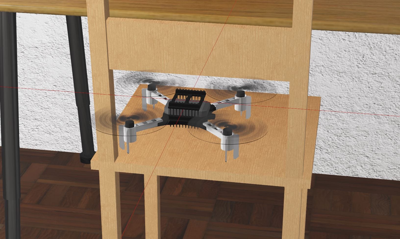
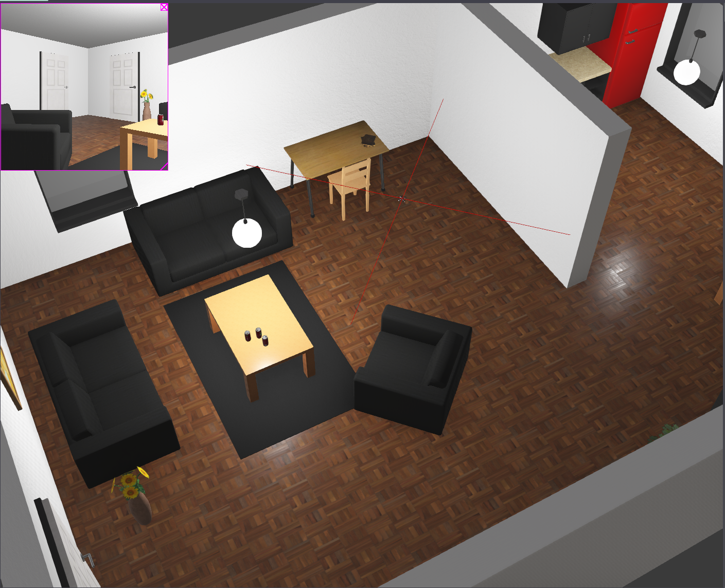
Some documentation I encountered mentioned potential compatibility issues with newer versions of Webots. If you run into this problem, Webots includes several built-in demos you can copy, including an apartment wall-following simulation.

Building my Initial Test Environment

I wanted something very simple to start with so I could begin developing my obstacle avoidance strategy without getting bogged down in complex world-building. My goal was to create a minimal viable test case that would let me focus on the important algorithmic work rather than spending weeks perfecting the simulation environment.

This approach led me to create a custom environment available at https://github.com/Engineering-Prowess/Basic-Webots-Crazyflie-Environment. The setup is deliberately simple: a single barrel positioned between clearly defined start and end zones.

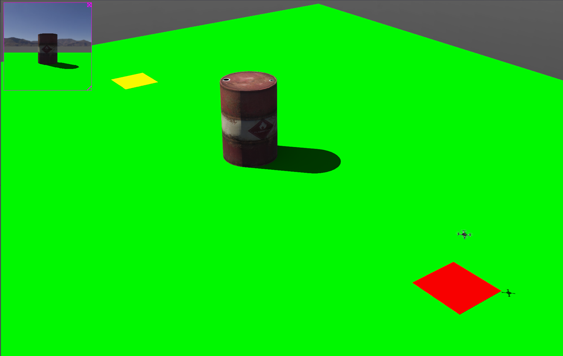
The beauty of this simple setup is that it forces me to solve the core problem: detecting an obstacle and planning a path around it. There are no distractions from multiple obstacles, complex geometries, or environmental complications. If I can't make the drone reliably navigate around a single barrel, there's no point in tackling more complex scenarios.

The environment includes:

• A clearly marked starting zone where the drone spawns
• A target zone the drone needs to reach
• A single cylindrical obstacle (barrel) positioned to block the direct path
• Adequate space for manoeuvring around the obstacle

Configuring the Simulation to Match Real Hardware

Before diving into algorithm development, I needed to ensure the simulated Crazyflie matched my actual hardware configuration. The default simulation includes sensors that I don't have on my physical drone, like GPS positioning, which would provide capabilities not available in the real world.

My real-world setup includes:

• Crazyflie 2.1 with AI deck for camera vision
• BMI088 IMU (accelerometer and gyroscope) and BMP388 pressure sensor
• Optical flow deck for position estimation
• No GPS or external positioning systems

Rather than modifying the simulation to disable these extra sensors, I will simply configure my algorithms to not use the GPS data that's available in Webots directly. This approach ensures that any navigation algorithms I develop will work with the same sensor limitations I'll face in the real world, while still allowing me to validate the approach if needed by temporarily enabling GPS for debugging.

The Crazyflie 2.1 comes with a BMI088 IMU that provides accelerometer and gyroscope data, along with a BMP388 pressure sensor for altitude estimation. The optical flow deck adds a VL53L1x Time-of-Flight (ToF) sensor for precise distance measurement up to 4 meters and a PMW3901 optical flow sensor that tracks movement relative to the ground by analyzing surface patterns. This combination provides sufficient positioning data for indoor obstacle avoidance tasks, though it works best over textured surfaces rather than blank floors.

Simulating the Optical Flow Deck

One challenge I encountered was how to simulate the optical flow deck's behaviour in Webots. The PMW3901 sensor outputs X and Y pixel displacement values that represent movement relative to the ground, essentially providing velocity estimates in the horizontal plane. However, Webots doesn't have a built-in PMW3901 optical flow sensor simulation.

My approach will be to use the GPS sensor data that's available in Webots, but process it to mimic the optical flow sensor's output characteristics. Instead of using absolute GPS coordinates directly, I calculate the velocity by taking derivatives of the position data and then add appropriate noise and limitations to match the optical flow sensor's behaviour.

The real PMW3901 sensor provides:

• X and Y displacement in pixels per frame
• Frame rates up to 121 FPS
• Minimum reliable operating height >80mm to approximately 1-2m
• Best performance on textured surfaces

In simulation, I will convert the GPS-derived velocity data to simulate these pixel displacement values, Ideally including the sensor's limitations like reduced accuracy on smooth surfaces and potential tracking failures. This is going to have to be addressed when moving to physical hardware.

Initial Observations and Next Steps

Running the basic simulation confirmed that the Webots handles our basic scenario for the Crazyflie. This simulation environment will serve as my testbed for developing the computer vision and path planning algorithms. The plan is to:

1. Implement basic obstacle detection using the simulated camera feed
2. Develop path planning algorithms to navigate around detected obstacles
3. Test different approaches to see which performs best in this controlled environment
4. Gradually increase complexity once the basic case works reliably

The next challenge will be integrating the camera feed from the simulation with the obstacle detection algorithms. While I wait for the real hardware streaming issues to be resolved, this simulated environment should let me make substantial progress on the core algorithms.

One advantage of this approach is that I can easily modify the obstacle positions, add multiple obstacles, or change the environment geometry to test different scenarios. Once the basic algorithms are working in simulation, transitioning to the real hardware should be much more straightforward.